参考莫烦的B站教程20，利用tensorflow自带的可视化工具tensorboard，在Google浏览器上进行了简单神网路的可视化。

一、将神经网络的结构可视化。

例子代码如下（spyder(tensorflow)编辑）：

Created on Mon Sep 17 18:37:22 2018

@author: Administrator
"""

# -*- coding: utf-8 -*-
"""
Created on Thu Sep 13 19:36:15 2018
莫烦B站的教学视频P16的例子。拟合一个二次函数。构建了一个隐藏层含有具有十个神经元的三层神经网络。激励函数用的relu
本次主要是演示将神经网络架构在tensorboard上进行可视化。
@author: Administrator
"""

import tensorflow as tf
#import matplotlib.pyplot as plt#首先加载可视化模块


def add_layer(inputs,in_size,out_size,activation_function=None):#None的话，默认就是线性函数
    with tf.name_scope('layer'):
        with tf.name_scope('weights'):
            Weights=tf.Variable(tf.random_normal([in_size,out_size]),name='W')#生成In_size行和out_size列的矩阵。代表权重矩阵。
        with tf.name_scope('biases'):
            biases=tf.Variable(tf.zeros([1,out_size])+0.1,name='b')
        with tf.name_scope('Wx_plus_b'):
            Wx_plus_b=tf.matmul(inputs,Weights)+biases#预测出来的还没有被激活的值存储在这个变量中。
        if activation_function is None:
            outputs=Wx_plus_b  
        else:
            outputs=activation_function(Wx_plus_b)
        return outputs#outputs是add_layer的输出值。
#define placeholder for inputs to network.
with tf.name_scope('inputs'):#input 包含了x和Y的input
    xs=tf.placeholder(tf.float32,[None,1],name='x_input')#1是x_data的属性为1.None指无论给多少个例子都ok。
    ys=tf.placeholder(tf.float32,[None,1],name='y_input')

#开始建造第一层layer。典型的三层神经网络：输入层（有多少个输入的x_data就有多少个神经元，本例中，只有一个属性，所以只有一个神经元输入），假设10个神经元的隐藏层，输出层。
#由于在使用relu，该代码就是用十条线段拟合一个抛物线。
l1=add_layer(xs,1,10,activation_function=tf.nn.relu)#L1仅是单隐藏层，全连接网络。

#再定义一个输出层,即:prediction
#add_layer的输出值是l1，把l1放在prediction的input。input的size就是隐藏层的size：10.output的size就是y_data的size就是1.
prediction=add_layer(l1,10,1,activation_function=None)
with tf.name_scope('loss'):
    loss=tf.reduce_mean(tf.reduce_sum(tf.square(ys-prediction),
                           reduction_indices=[1]))#reduction_indices=[1]:按行求和。reduction_indices=[0]按列求和。sum是将所有例子求和，再求平均（mean）。
with tf.name_scope('train'):
#通过训练学习。提升误差。
    train_step=tf.train.GradientDescentOptimizer(0.1).minimize(loss)#以0.1的学习效率来训练学习，来减小loss。
sess=tf.Session()
writer=tf.summary.FileWriter('logs',sess.graph)#把图片load到log的文件夹里，在浏览器里浏览。
#important step
sess.run(tf.global_variables_initializer())

期间，需要注意的是：

@1、将代码run之后，创建的log文件被放在了spyer的.py文件的默认保存位置。因此下一步在cmd上执行：

”tensorboard --logdir=logs“（win10平台上需要这样写，而不是logdir='logs/'）时，需要将cmd的工作路径改到“log”文件所在的上一级。

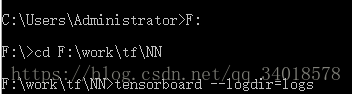
@2、根据给出的地址即at后面的地址，copy到Google浏览器ernter后，会进入到tensorboard的在线界面：

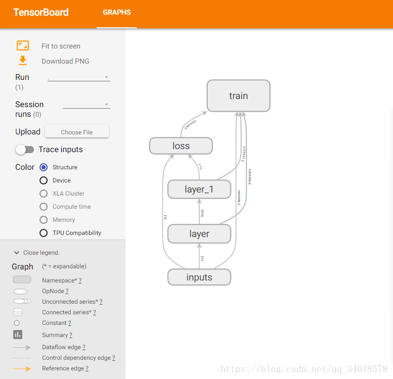
二、将各个值以及Loss的变化曲线可视化。示例代码如下：

# -*- coding: utf-8 -*-
"""
Created on Mon Sep 17 18:37:22 2018

@author: Administrator
"""

# -*- coding: utf-8 -*-
"""
Created on Thu Sep 13 19:36:15 2018
莫烦B站的教学视频P16的例子。拟合一个二次函数。构建了一个隐藏层含有具有十个神经元的三层神经网络。激励函数用的relu
本次主要是演示将神经网络运行时候内部的参数以及Loss的变化曲线在tensorboard上进行可视化。
@author: Administrator
"""

import tensorflow as tf
#import matplotlib.pyplot as plt#首先加载可视化模块
import numpy as np

def add_layer(inputs,in_size,out_size,n_layer,activation_function=None):#None的话，默认就是线性函数
    #add one more layer and return the output of this layer
    layer_name='layer%s'%n_layer
    with tf.name_scope(layer_name):
        with tf.name_scope('weights'):
            Weights=tf.Variable(tf.random_normal([in_size,out_size]),name='W')#生成In_size行和out_size列的矩阵。代表权重矩阵。
            tf.summary.histogram(layer_name+'/weights',Weights)
        with tf.name_scope('biases'):
            biases=tf.Variable(tf.zeros([1,out_size])+0.1,name='b')
            tf.summary.histogram(layer_name+'/biases',biases)
        with tf.name_scope('Wx_plus_b'):
            Wx_plus_b=tf.matmul(inputs,Weights)+biases#预测出来的还没有被激活的值存储在这个变量中。
        if activation_function is None:
            outputs=Wx_plus_b  
        else:
            outputs=activation_function(Wx_plus_b)
        tf.summary.histogram(layer_name+'/outputs',outputs)
        return outputs#outputs是add_layer的输出值。
#define placeholder for inputs to network.
#make up some real data
x_data=np.linspace(-1,1,300)[:,np.newaxis]
noise=np.random.normal(0,0.05,x_data.shape)
y_data=np.square(x_data)-0.5+noise
with tf.name_scope('inputs'):#input 包含了x和Y的input
    xs=tf.placeholder(tf.float32,[None,1],name='x_input')#1是x_data的属性为1.None指无论给多少个例子都ok。
    ys=tf.placeholder(tf.float32,[None,1],name='y_input')

#开始建造第一层layer。典型的三层神经网络：输入层（有多少个输入的x_data就有多少个神经元，本例中，只有一个属性，所以只有一个神经元输入），假设10个神经元的隐藏层，输出层。
#由于在使用relu，该代码就是用十条线段拟合一个抛物线。
l1=add_layer(xs,1,10,n_layer=1,activation_function=tf.nn.relu)#L1仅是单隐藏层，全连接网络。

#再定义一个输出层,即:prediction
#add_layer的输出值是l1，把l1放在prediction的input。input的size就是隐藏层的size：10.output的size就是y_data的size就是1.
prediction=add_layer(l1,10,1,n_layer=2,activation_function=None)
with tf.name_scope('loss'):
    loss=tf.reduce_mean(tf.reduce_sum(tf.square(ys-prediction),
                           reduction_indices=[1]))#reduction_indices=[1]:按行求和。reduction_indices=[0]按列求和。sum是将所有例子求和，再求平均（mean）。
    tf.summary.scalar('loss',loss)#loss这里要用scalar。如果是在减小，说明学到东西了。
with tf.name_scope('train'):
#通过训练学习。提升误差。
    train_step=tf.train.GradientDescentOptimizer(0.1).minimize(loss)#以0.1的学习效率来训练学习，来减小loss。
sess=tf.Session()
merged=tf.summary.merge_all()
writer=tf.summary.FileWriter('logs',sess.graph)#把图片load到log的文件夹里，在浏览器里浏览。
#important step
sess.run(tf.global_variables_initializer())
for i in range(500):
     sess.run(train_step,feed_dict={xs:x_data,ys:y_data})
     if i%50==0:
         result=sess.run(merged,
                         feed_dict={xs:x_data,ys:y_data})
         writer.add_summary(result,i)

期间遇到如下问题：

@1、因tensorflow版本原因，很多函数不一样，报错。大概总结如下：

除特别声明，本站所有文章均为原创，如需转载请以超级链接形式注明出处：SmartCat's Blog